Table Of Content
- Factorial Fit: LOGT versus B, C, D
- Book traversal links for Lesson 5: Introduction to Factorial Designs
- Creating a Factorial Design in Minitab
- Sequential Procedure for Strategically Finding a Model
- A Complete Guide: The 2×2 Factorial Design
- A catalogue of three-level regular fractional factorial designs
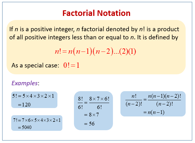
- Notation
Statology Study is the ultimate online statistics study guide that helps you study and practice all of the core concepts taught in any elementary statistics course and makes your life so much easier as a student. In the previous plot, the two lines were roughly parallel so there is likely no interaction effect between watering frequency and sunlight exposure. The other approach is a weighted analysis, where you weight the observations according to the inverse of their variance.
Factorial Fit: LOGT versus B, C, D
But they might choose to treat time of day as a between-subjects factor by testing each participant either during the day or during the night (perhaps because this only requires them to come in for testing once). Thus each participant in this mixed design would be tested in two of the four conditions. In the remainder of this section, we will focus on between-subjects factorial designs only. Also, regardless of the design, the actual assignment of participants to conditions is typically done randomly. Just as including multiple levels of a single independent variable allows one to answer more sophisticated research questions, so too does including multiple independent variables in the same experiment.
Book traversal links for Lesson 5: Introduction to Factorial Designs
This would be a 2 x 2 x 2 factorial design and would have eight conditions. In practice, it is unusual for there to be more than three independent variables with more than two or three levels each. In Chapter 1 we briefly described a study conducted by Simone Schnall and her colleagues, in which they found that washing one’s hands leads people to view moral transgressions as less wrong [SBH08]. In a different but related study, Schnall and her colleagues investigated whether feeling physically disgusted causes people to make harsher moral judgments [SHCJ08].
Creating a Factorial Design in Minitab
First, non-manipulated independent variables are usually participant characteristics (private body consciousness, hypochondriasis, self-esteem, and so on), and as such they are, by definition, between-subject factors. For example, people are either low in hypochondriasis or high in hypochondriasis; they cannot be in both of these conditions. In a between-subjects factorial design, all of the independent variables are manipulated between subjects. For example, all participants could be tested either while using a cell phone or while not using a cell phone and either during the day or during the night.
Sequential Procedure for Strategically Finding a Model
The dependent variable is the light (we measure whether it is on or off). The first independent variable is light switch #1, and it has two levels, up or down. The second independent variable is light switch #2, and it also has two levels, up or down. When there are two independent variables, each with two levels, there are four total conditions that can be tested.
A Complete Guide: The 2×2 Factorial Design
It is true that correlational research cannot unambiguously establish that one variable causes another. Complex correlational research, however, can often be used to rule out other plausible interpretations. Research findings are often presented to readers using graphs or tables. For example, the very same pattern of data can be displayed in a bar graph, line graph, or table of means. These different formats can make the data look different, even though the pattern in the data is the same. An important skill to develop is the ability to identify the patterns in the data, regardless of the format they are presented in.
A catalogue of three-level regular fractional factorial designs
The columns for AB, AC and BC represent the corresponding two-factor interactions. The columns for A, B and C represent the corresponding main effects, as the entries in each column depend only on the level of the corresponding factor. For example, the entries in the B column follow the same pattern as the middle component of "cell", as can be seen by sorting on B.
Novel coil design and analysis for high-power wireless power transfer with enhanced Q-factor Scientific Reports - Nature.com
Novel coil design and analysis for high-power wireless power transfer with enhanced Q-factor Scientific Reports.
Posted: Tue, 14 Mar 2023 07:00:00 GMT [source]
From the example above, suppose you find that as dosage increases, the percentage of people who suffer from seizures increases as well. You also notice that age does not play a role; both 20 and 40 year olds suffer the same percentage of seizures for a given amount of CureAll. From this information, you can conclude that the chance of a patient suffering a seizure is minimized at lower dosages of the drug (5 mg). The second graph illustrates that with increased drug dosage there is an increased percentage of seizures, while the first graph illustrates that with increased age there is no change in the percentage of seizures. Both of these graphs only contain one main effect, since only dose has an effect the percentage of seizures.
THE X FACTOR OF COLLECTIBLE DESIGN Community Savannah News, Events, Restaurants, Music - Connect Savannah.com
THE X FACTOR OF COLLECTIBLE DESIGN Community Savannah News, Events, Restaurants, Music.
Posted: Wed, 27 Apr 2022 07:00:00 GMT [source]
Notation
By the traditional experimentation, each experiment would have to be isolated separately to fully find the effect on B. This would have resulted in 8 different experiments being performed. Note that only four experiments were required in factorial designs to solve for the eight values in A and B. Researchers often use factorial designs to understand the causal influences behind the effects they are interested in improving. Effects are the change in a measure (DV) caused by a manipulation (IV levels). In addition, the efficiency of a factorial experiment depends in part on the extent to which higher order interactions are not found.
This is simply a plot that can quickly show you what is important. It looks at the size of the effects and plots the effect size on a horizontal axis ranked from largest to smallest effect. To summarize what we have learned in this lesson thus far, we can write a contrast of the totals which defines an effect, we can estimate the variance for this effect and we can write the sum of squares for an effect. We can do this very simply using Yates notation which historically has been the value of using this notation. We use "(1)" to denote that both factors are at the low level, "a" for when A is at its high level and B is at its low level, "b" for when B is at its high level and A is at its low level, and "ab" when both A and B factors are at their high level.
In other words, we want to find out what other IVs might affect the size of the distraction effect (make it bigger or smaller, or even flip around!). If our distraction manipulation is super-distracting, then what should we expect to find when we compare spot-the-difference performance between the no-distraction and distraction conditions? If our manipulation works, then we should find that people find more differences when they are not distracted, and less differences when they are distracted. Factorial designs are the basis for another important principle besides blocking - examining several factors simultaneously.
This can pose interpretive challenges as it may be difficult to separate the effects of a component per se from the impact of burden. The advantage of multiple regression is that it can show whether an independent variable makes a contribution to a dependent variable over and above the contributions made by other independent variables. As a hypothetical example, imagine that a researcher wants to know how the independent variables of income and health relate to the dependent variable of happiness.
For example, measures of warmth, gregariousness, activity level, and positive emotions tend to be highly correlated with each other and are interpreted as representing the construct of extraversion. As a final example, researchers Peter Rentfrow and Samuel Gosling asked more than 1,700 university students to rate how much they liked 14 different popular genres of music [RG03]. They then submitted these 14 variables to a factor analysis, which identified four distinct factors. The simplest way to understand a main effect is to pretend that the other independent variables do not exist. If you do this, then you simply have a single-factor design, and you are asking whether that single factor caused change in the measurement. For a 2x2 experiment, you do this twice, once for each independent variable.


No comments:
Post a Comment